NBLAST
NBLAST is a method to quantify morphological similarity.
Worked examples
Session 5 · Similarity / NBLAST on the VFB Self-led Learning Sessions works through this against live VFB data, in Python, R, an MCP-capable assistant, VFB Chat and the 3D browser. Free, self-paced and open to anyone.
Overview
NBLAST (Costa et al., 2016) is a method to quantify morphological similarity. It works on “dotprops” which represent neurons as tangent vectors. For each tangent vector in the query neuron, NBLAST finds the closest tangent vector in the target neuron and calculates a score from the distance between and the dotproduct of the two vectors. The final NBLAST score is the sum over all query-target vector pairs. Typically, this score is normalized to a self-self comparison (i.e. a perfect match would be 1).

Finding Matching Neurons
VFB computes NBLAST scores for all neurons in its database. So if all you want is a list of similar neurons, it’s fastest (and easiest) to get those directly from VFB.
# Import libs and initialise API objects
from vfb_connect.cross_server_tools import VfbConnect
import navis.interfaces.neuprint as neu
import pandas as pd
import navis
navis.set_pbars(jupyter=False)
vc = VfbConnect()
client = neu.Client('https://neuprint.janelia.org', dataset='hemibrain:v1.1')
First let’s write a function to grab VFB neurons and turn them into navis neurons. This is modified from vc.neo_query_wrapper.get_images.
import requests
from tqdm import tqdm
def get_vfb_neurons(vfb_ids, template='JRC2018Unisex'):
"""Load neurons from VFB as navis.TreeNeurons."""
vfb_ids = list(navis.utils.make_iterable(vfb_ids))
inds = vc.neo_query_wrapper.get_anatomical_individual_TermInfo(short_forms=vfb_ids)
nl = []
# Note: queries should be parallelized in the future
# -> for pymaid I use request-futures which works really well
for i in tqdm(inds, desc='Loading VFB neurons', leave=False):
if not ('has_image' in i['term']['core']['types']):
continue
label = i['term']['core']['label']
image_matches = [x['image'] for x in i['channel_image']]
if not image_matches:
continue
for imv in image_matches:
if imv['template_anatomy']['label'] == template:
r = requests.get(imv['image_folder'] + '/volume.swc')
### Slightly dodgy warning - could mask network errors
if not r.ok:
warnings.warn("No '%s' file found for '%s'." % (image_type, label))
continue
# `id` should ideally be unique but that's not enforced
n = navis.TreeNeuron(r.text, name=label, id=i['term']['core']['short_form'])
# This registers attributes that you want to show in the summary
# alternatively we could have a generic attribute like so:
# n.template = template
n._register_attr("template", template, temporary=False)
# I assume all available templates are in microns?
# @Robbie -do we have this metadata on templates? If not, we should add ASAP.
n.units = '1 micron'
nl.append(n)
return navis.NeuronList(nl)
# Search for similar neurons using the VFB ID of an ellipsoid body neuron in FAFB
# We got that ID from a search on the VFB website
similar_to_EPG6L1 = vc.get_similar_neurons('VFB_001012ay')
similar_to_EPG6L1
| id | NBLAST_score | label | types | source_id | accession_in_source | |
|---|---|---|---|---|---|---|
| 0 | VFB_jrchjtk6 | 0.525 | EPG(PB08)_L6 - 541870397 | [EB-PB 1 glomerulus-D/Vgall neuron] | neuprint_JRC_Hemibrain_1point1 | 541870397 |
| 1 | VFB_jrchjtk8 | 0.524 | EPG(PB08)_L6 - 912601268 | [EB-PB 1 glomerulus-D/Vgall neuron] | neuprint_JRC_Hemibrain_1point1 | 912601268 |
| 2 | VFB_jrchjtkb | 0.504 | EPG(PB08)_L6 - 788794171 | [EB-PB 1 glomerulus-D/Vgall neuron] | neuprint_JRC_Hemibrain_1point1 | 788794171 |
| 3 | VFB_jrchjtji | 0.481 | EL(EQ5)_L - 1036753721 | [EBw.AMP.s-Dga-s.b neuron] | neuprint_JRC_Hemibrain_1point1 | 1036753721 |
# Read those neurons from VFB
query = get_vfb_neurons('VFB_001012ay')
matches = get_vfb_neurons(similar_to_EPG6L1.id.values)
matches
| type | name | id | n_nodes | n_connectors | n_branches | n_leafs | cable_length | soma | units | template | |
|---|---|---|---|---|---|---|---|---|---|---|---|
| 0 | navis.TreeNeuron | EPG(PB08)_L6 - 912601268 | VFB_jrchjtk8 | 9819 | None | 1000 | 1015 | 2211.292188 | None | 1 micron | JRC2018Unisex |
| 1 | navis.TreeNeuron | EL(EQ5)_L - 1036753721 | VFB_jrchjtji | 13864 | None | 1942 | 1974 | 3403.311508 | [1] | 1 micron | JRC2018Unisex |
| 2 | navis.TreeNeuron | EPG(PB08)_L6 - 788794171 | VFB_jrchjtkb | 9651 | None | 962 | 987 | 2125.364857 | None | 1 micron | JRC2018Unisex |
| 3 | navis.TreeNeuron | EPG(PB08)_L6 - 541870397 | VFB_jrchjtk6 | 11042 | None | 1099 | 1127 | 2432.101351 | [1] | 1 micron | JRC2018Unisex |
# Define colors such that query is black
import seaborn as sns
colors = ['k'] + sns.color_palette('muted', len(matches))
navis.plot3d([query, matches], color=colors)
These like a good match!
Clustering Groups of Neurons
Now imagine you have a set of neurons and you want to group them into morphologically similar “types”. To demonstrate this, we will take some ellipsoid body neurons from VFB and cluster them using NBLAST.
# Find instances of EB-PB-gall neurons
eb_pb_ids = pd.DataFrame.from_records(vc.get_instances("adult ellipsoid body-protocerebral bridge-gall neuron"))
eb_pb_ids.head()
| label | symbol | id | tags | parents_label | parents_id | data_source | accession | templates | dataset | license | |
|---|---|---|---|---|---|---|---|---|---|---|---|
| 0 | EPGt(PB09)_L9 - 1168664447 | VFB_jrchjtlc | Entity|has_image|Adult|Anatomy|has_neuron_conn... | EB slice 8-GA-PB slice 9 neuron | FBbt_00111423 | neuprint_JRC_Hemibrain_1point1 | 1168664447 | JRC_FlyEM_Hemibrain|JRC2018Unisex | Xu2020NeuronsV1point1 | https://creativecommons.org/licenses/by/4.0/le... | |
| 1 | EPGt(PB09)_R9 - 1219069439 | VFB_jrchjtl9 | Entity|has_image|Adult|Anatomy|has_neuron_conn... | EB slice 8-GA-PB slice 9 neuron | FBbt_00111423 | neuprint_JRC_Hemibrain_1point1 | 1219069439 | JRC2018Unisex|JRC_FlyEM_Hemibrain | Xu2020NeuronsV1point1 | https://creativecommons.org/licenses/by/4.0/le... | |
| 2 | EPG(PB08)_L2 - 697001770 | VFB_jrchjtkw | Entity|has_image|Adult|Anatomy|has_neuron_conn... | EB-PB 1 glomerulus-D/Vgall neuron | FBbt_00047030 | neuprint_JRC_Hemibrain_1point1 | 697001770 | JRC2018Unisex|JRC_FlyEM_Hemibrain | Xu2020NeuronsV1point1 | https://creativecommons.org/licenses/by/4.0/le... | |
| 3 | EPG(PB08)_R8 - 1125964814 | VFB_jrchjtl5 | Entity|has_image|Adult|Anatomy|has_neuron_conn... | EB-PB 1 glomerulus-D/Vgall neuron | FBbt_00047030 | neuprint_JRC_Hemibrain_1point1 | 1125964814 | JRC2018Unisex|JRC_FlyEM_Hemibrain | Xu2020NeuronsV1point1 | https://creativecommons.org/licenses/by/4.0/le... | |
| 4 | EPG(PB08)_L6 - 912601268 | VFB_jrchjtk8 | Entity|has_image|Adult|Anatomy|has_neuron_conn... | EB-PB 1 glomerulus-D/Vgall neuron | FBbt_00047030 | neuprint_JRC_Hemibrain_1point1 | 912601268 | JRC2018Unisex|JRC_FlyEM_Hemibrain | Xu2020NeuronsV1point1 | https://creativecommons.org/licenses/by/4.0/le... |
# Get the neurons from VFB
eb_pb = get_vfb_neurons(eb_pb_ids.id.values)
eb_pb
Loading VFB neurons: 100%|██████████| 62/62 [01:04<00:00, 1.04s/it]
| type | name | id | n_nodes | n_connectors | n_branches | n_leafs | cable_length | soma | units | |
|---|---|---|---|---|---|---|---|---|---|---|
| 0 | navis.TreeNeuron | EPG(PB08)_R5 - 725951521 | VFB_jrchjtk5 | 11097 | None | 1223 | 1251 | 2221.279929 | [1] | 1 dimensionless |
| 1 | navis.TreeNeuron | EPG(PB08)_R2 - 632544268 | VFB_jrchjtkt | 12861 | None | 1475 | 1507 | 2664.323311 | [1] | 1 dimensionless |
| ... | ... | ... | ... | ... | ... | ... | ... | ... | ... | ... |
| 60 | navis.TreeNeuron | EPG(PB08)_R5 - 694920753 | VFB_jrchjtk7 | 11358 | None | 1348 | 1376 | 2335.616245 | [1] | 1 dimensionless |
| 61 | navis.TreeNeuron | EPG(PB08)_R6 - 910438331 | VFB_jrchjtkc | 10983 | None | 1086 | 1107 | 2340.485198 | [1] | 1 dimensionless |
Now that we have the skeletons, we need to turn them into dotprops. Keep in mind that:
- NBLAST is optimized for data in microns. Since our neurons are in the
JRC2018Unisextemplate, they already are. - Neurons should have the same sampling rate (i.e. nodes per micron). To ensure this we will resample the neurons to 1 point per micron.
- We won’t be doing this this time around but we typically simplify the neurons slightly by e.g. pruning small twigs (
navis.prune_twigs()) to reduce noise.
eb_dps = navis.make_dotprops(eb_pb, resample=1, k=5)
# Note this NeuronList /contains dotprops now
eb_dps
| type | name | id | k | units | n_points | |
|---|---|---|---|---|---|---|
| 0 | navis.Dotprops | EPG(PB08)_R5 - 725951521 | VFB_jrchjtk5 | 5 | 1 dimensionless | 2683 |
| 1 | navis.Dotprops | EPG(PB08)_R2 - 632544268 | VFB_jrchjtkt | 5 | 1 dimensionless | 3152 |
| ... | ... | ... | ... | ... | ... | ... |
| 60 | navis.Dotprops | EPG(PB08)_R5 - 694920753 | VFB_jrchjtk7 | 5 | 1 dimensionless | 2924 |
| 61 | navis.Dotprops | EPG(PB08)_R6 - 910438331 | VFB_jrchjtkc | 5 | 1 dimensionless | 2486 |
To illustrate what dotprops are, lets visualize one side-by-side with its skeleton.
sk = eb_pb[0].copy()
dp = eb_dps[0].copy()
# Slightly offset the dotprops by a micron
dp.points[:, 0] += 1
navis.plot3d([sk, dp], color=['k', 'r'])
Now we can run the NBLAST. Note that in this case, we run an all-by-all NBLAST which means that we don’t need to worry about the directionality - i.e. whether we NBLAST A->B or B->A.
scores = navis.nblast_allbyall(eb_dps)
scores.head()
| VFB_jrchjtk5 | VFB_jrchjtkt | VFB_001012ba | VFB_jrchjtkj | VFB_jrchjtkp | VFB_jrchjtke | VFB_jrchjtkr | VFB_jrchjtkb | VFB_00004319 | VFB_00009714 | ... | VFB_jrchjtk8 | VFB_001012bp | VFB_jrchjtk9 | VFB_jrchjtki | VFB_jrchjtl3 | VFB_jrchjtkv | VFB_001012b9 | VFB_001012bb | VFB_jrchjtk7 | VFB_jrchjtkc | |
|---|---|---|---|---|---|---|---|---|---|---|---|---|---|---|---|---|---|---|---|---|---|
| VFB_jrchjtk5 | 1.000000 | -0.083960 | 0.427659 | 0.058210 | 0.021904 | 0.484210 | 0.168235 | 0.178954 | 0.065457 | 0.355732 | ... | 0.130788 | 0.528314 | 0.569923 | -0.029195 | -0.130578 | -0.072185 | 0.381668 | 0.139970 | 0.816455 | 0.504740 |
| VFB_jrchjtkt | -0.062465 | 1.000000 | -0.030980 | -0.124326 | 0.507521 | -0.122518 | -0.143298 | 0.091243 | -0.124431 | -0.142560 | ... | 0.172337 | -0.059201 | 0.078412 | -0.116040 | 0.129102 | -0.034670 | -0.053382 | 0.103465 | -0.063922 | -0.073508 |
| VFB_001012ba | 0.129771 | -0.115879 | 1.000000 | 0.374231 | -0.091531 | 0.549519 | 0.450368 | -0.130200 | 0.161574 | 0.112378 | ... | -0.127990 | 0.786001 | 0.013910 | 0.330330 | -0.000875 | 0.212914 | 0.817302 | -0.110084 | 0.200497 | 0.569953 |
| VFB_jrchjtkj | -0.027448 | -0.219602 | 0.483341 | 1.000000 | -0.031111 | 0.443643 | 0.461981 | -0.025682 | 0.061803 | 0.434210 | ... | -0.034895 | 0.389407 | -0.091165 | 0.819716 | 0.217721 | 0.552982 | 0.447278 | -0.053055 | 0.045722 | 0.485596 |
| VFB_jrchjtkp | -0.158602 | 0.493915 | -0.161524 | -0.103061 | 1.000000 | -0.212700 | -0.221368 | 0.405601 | -0.163415 | -0.130491 | ... | 0.515069 | -0.170831 | 0.024440 | -0.095100 | -0.032720 | -0.082523 | -0.182386 | 0.412998 | -0.158171 | -0.197676 |
5 rows × 62 columns
Next, we need to take those forward scores (A->B) and symmetrize by calculating mean scores (A<->B).
# Symmetrize scores
scores_mean = (scores + scores.T) / 2
scores_mean.head()
| VFB_jrchjtk5 | VFB_jrchjtkt | VFB_001012ba | VFB_jrchjtkj | VFB_jrchjtkp | VFB_jrchjtke | VFB_jrchjtkr | VFB_jrchjtkb | VFB_00004319 | VFB_00009714 | ... | VFB_jrchjtk8 | VFB_001012bp | VFB_jrchjtk9 | VFB_jrchjtki | VFB_jrchjtl3 | VFB_jrchjtkv | VFB_001012b9 | VFB_001012bb | VFB_jrchjtk7 | VFB_jrchjtkc | |
|---|---|---|---|---|---|---|---|---|---|---|---|---|---|---|---|---|---|---|---|---|---|
| VFB_jrchjtk5 | 1.000000 | -0.073212 | 0.278715 | 0.015381 | -0.068349 | 0.411257 | 0.098761 | 0.142277 | 0.032064 | 0.187264 | ... | 0.070828 | 0.437337 | 0.572156 | -0.043306 | -0.140155 | -0.092071 | 0.271765 | 0.131925 | 0.820455 | 0.398975 |
| VFB_jrchjtkt | -0.073212 | 1.000000 | -0.073429 | -0.171964 | 0.500718 | -0.142672 | -0.164992 | 0.062182 | -0.115399 | -0.162311 | ... | 0.176281 | -0.099006 | 0.074666 | -0.162002 | 0.097262 | -0.082222 | -0.089534 | 0.120931 | -0.075555 | -0.114645 |
| VFB_001012ba | 0.278715 | -0.073429 | 1.000000 | 0.428786 | -0.126527 | 0.667980 | 0.527915 | -0.128599 | 0.220682 | 0.068423 | ... | -0.143015 | 0.792216 | 0.070675 | 0.389590 | 0.018090 | 0.176492 | 0.826461 | -0.102122 | 0.332148 | 0.684591 |
| VFB_jrchjtkj | 0.015381 | -0.171964 | 0.428786 | 1.000000 | -0.067086 | 0.436914 | 0.494708 | -0.031511 | -0.030539 | 0.489038 | ... | -0.045253 | 0.396773 | -0.069074 | 0.824681 | 0.168068 | 0.508538 | 0.395092 | -0.062799 | 0.100087 | 0.509110 |
| VFB_jrchjtkp | -0.068349 | 0.500718 | -0.126527 | -0.067086 | 1.000000 | -0.164867 | -0.203583 | 0.413305 | -0.171488 | -0.124160 | ... | 0.537125 | -0.109346 | 0.020020 | -0.074199 | -0.011358 | -0.093459 | -0.133473 | 0.435029 | -0.062292 | -0.161714 |
5 rows × 62 columns
From here on out, we use cookie cutter scipy to produce a hierarchical clustering. First we need to convert those similarity scores to distances because that’s what scipy operates on:
dist_mean = (scores_mean - 1) * -1
dist_mean.head()
| VFB_jrchjtk5 | VFB_jrchjtkt | VFB_001012ba | VFB_jrchjtkj | VFB_jrchjtkp | VFB_jrchjtke | VFB_jrchjtkr | VFB_jrchjtkb | VFB_00004319 | VFB_00009714 | ... | VFB_jrchjtk8 | VFB_001012bp | VFB_jrchjtk9 | VFB_jrchjtki | VFB_jrchjtl3 | VFB_jrchjtkv | VFB_001012b9 | VFB_001012bb | VFB_jrchjtk7 | VFB_jrchjtkc | |
|---|---|---|---|---|---|---|---|---|---|---|---|---|---|---|---|---|---|---|---|---|---|
| VFB_jrchjtk5 | -0.000000 | 1.073212 | 0.721285 | 0.984619 | 1.068349 | 0.588743 | 0.901239 | 0.857723 | 0.967936 | 0.812736 | ... | 0.929172 | 0.562663 | 0.427844 | 1.043306 | 1.140155 | 1.092071 | 0.728235 | 0.868075 | 0.179545 | 0.601025 |
| VFB_jrchjtkt | 1.073212 | -0.000000 | 1.073429 | 1.171964 | 0.499282 | 1.142672 | 1.164992 | 0.937818 | 1.115399 | 1.162311 | ... | 0.823719 | 1.099006 | 0.925334 | 1.162002 | 0.902738 | 1.082222 | 1.089534 | 0.879069 | 1.075555 | 1.114645 |
| VFB_001012ba | 0.721285 | 1.073429 | -0.000000 | 0.571214 | 1.126527 | 0.332020 | 0.472085 | 1.128599 | 0.779318 | 0.931577 | ... | 1.143015 | 0.207784 | 0.929325 | 0.610410 | 0.981910 | 0.823508 | 0.173539 | 1.102122 | 0.667852 | 0.315409 |
| VFB_jrchjtkj | 0.984619 | 1.171964 | 0.571214 | -0.000000 | 1.067086 | 0.563086 | 0.505292 | 1.031511 | 1.030539 | 0.510962 | ... | 1.045253 | 0.603227 | 1.069074 | 0.175319 | 0.831932 | 0.491462 | 0.604908 | 1.062799 | 0.899913 | 0.490890 |
| VFB_jrchjtkp | 1.068349 | 0.499282 | 1.126527 | 1.067086 | -0.000000 | 1.164867 | 1.203583 | 0.586695 | 1.171488 | 1.124160 | ... | 0.462875 | 1.109346 | 0.979980 | 1.074199 | 1.011358 | 1.093459 | 1.133473 | 0.564971 | 1.062292 | 1.161714 |
5 rows × 62 columns
from scipy.spatial.distance import squareform
from scipy.cluster.hierarchy import linkage, dendrogram, fcluster
# This turns the square distance matrix into 1-d vector form
dist_sq = squareform(dist_mean)
# This does the actual hierarchical clustering
Z = linkage(dist_sq, method='ward', optimal_ordering=True)
# Plot a quick dendrogram
import matplotlib.pyplot as plt
import seaborn as sns
# Generate the canvas
fig, ax = plt.subplots(figsize=(12, 5))
# Make some more meaningful labels
vfb2name = dict(zip(eb_pb.id, eb_pb.name))
labels = dist_mean.index.map(lambda x: vfb2name[x].split(' - ')[0])
# Plot the dendrogram
dn = dendrogram(Z, ax=ax, labels=labels, color_threshold=.65, above_threshold_color='lightgrey')
# Make xticks biggger
ax.set_xticklabels(ax.get_xticklabels(), size=11)
# Clean axes
sns.despine(bottom=True)
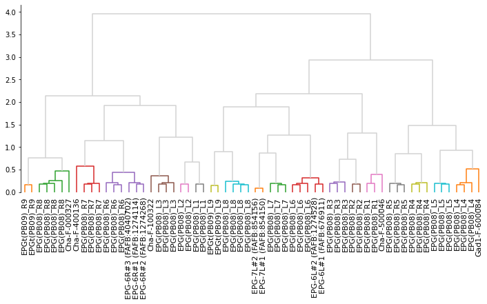
# Make cluster matching the color threshold in the dendrogram
clusters = fcluster(Z, t=.65, criterion='distance')
clusters
array([16, 14, 4, 5, 11, 4, 3, 12, 2, 19, 13, 4, 8, 3, 19, 2, 5,
13, 3, 11, 17, 14, 16, 6, 12, 15, 18, 11, 12, 15, 15, 18, 5, 10,
9, 2, 19, 8, 1, 9, 19, 3, 1, 10, 2, 9, 7, 18, 9, 2, 17,
13, 12, 4, 17, 5, 7, 6, 4, 12, 16, 4], dtype=int32)
# We have to downsample the neurons for visualization
# because DeepNote enforces a limit on the size of plots
eb_pb_ds = eb_pb.downsample(10)
# Make a color per cluster
palette = sns.color_palette('tab20', max(clusters))
cmap = dict(zip(range(1, max(clusters) + 1), palette))
colors = [cmap[i] for i in clusters]
navis.plot3d(eb_pb_ds, color=colors)